Anderson-Sleath yield curves: latest and historical

The Bank of England publishes daily fitted yield curves at all maturities using the Anderson and Sleath (2001) smoothing methodology. Five curves are produced: nominal gilt, real (index-linked) gilt, implied inflation, overnight index swap (OIS), and the commercial bank liability curve (BLC). Each is available in spot and instantaneous-forward form.

The default behaviour of boe_curve() returns the latest published month, matching what most analysts need when they reach for “today’s curve”. Pass from, to, or frequency = "monthly" and the function switches to the BoE historical archive, which extends back as far as 1979 for nominal gilts.

Latest published month

latest <- boe_curve(curve = "nominal", measure = "spot")
#> ℹ Downloading yield curve archive from Bank of England
#> ✔ Downloading yield curve archive from Bank of England [731ms]
#> 
range(latest$date)
#> [1] "2026-05-01" "2026-05-07"
range(latest$maturity_years)
#> [1]  0.5 40.0

boe_curve() returns a long-format boe_tbl with one row per (date, maturity) pair. Provenance is attached as an attribute:

attr(latest, "boe_query")$source
#> [1] "latest"
attr(latest, "boe_query")$series_codes
#> [1] "AS_NOMINAL_SPOT"

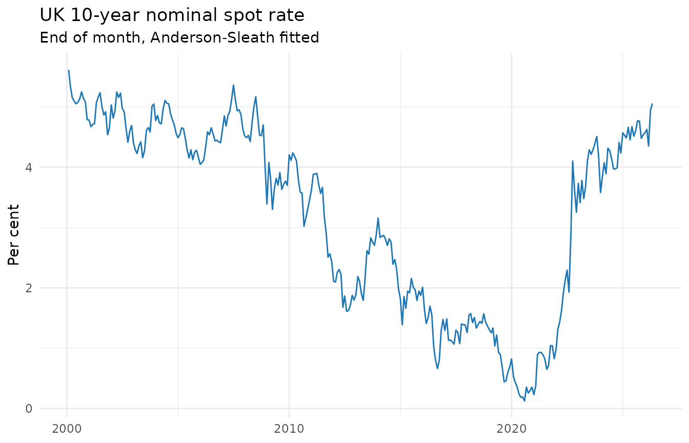
Historical: 10-year nominal spot rate since 2000

For time-series work, boe_curve_panel() reshapes the long format into a wide panel with one column per pillar maturity. End-of-month frequency is plenty for multi-decade work and keeps the download small.

panel <- boe_curve_panel(
  curve     = "nominal",
  measure   = "spot",
  frequency = "monthly",
  from      = "2000-01-01",
  maturities = c(2, 5, 10, 20)
)
#> ℹ Downloading nominal monthly yield-curve archive from Bank of England
#> ✔ Downloading nominal monthly yield-curve archive from Bank of England [156ms]
#> 
head(panel)
#> # BoE [boe_curve_panel]: 1 series [AS_NOMINAL_SPOT] · 6 obs · 2000-01-31 to 2026-04-30 · freq=monthly
#>         date       m2       m5      m10      m20
#> 1 2000-01-31 6.474909 6.286147 5.613887 4.478985
#> 2 2000-02-29 6.302563 6.010255 5.334982 4.363222
#> 3 2000-03-31 6.273430 5.857503 5.147789 4.349529
#> 4 2000-04-30 6.069206 5.704744 5.097727 4.262276
#> 5 2000-05-31 6.136496 5.695847 5.051332 4.304463
#> 6 2000-06-30 5.942865 5.594983 5.073053 4.379719

if (requireNamespace("ggplot2", quietly = TRUE)) {
  ggplot2::ggplot(panel, ggplot2::aes(date, m10)) +
    ggplot2::geom_line(colour = "#1f77b4") +
    ggplot2::labs(
      title    = "UK 10-year nominal spot rate",
      subtitle = "End of month, Anderson-Sleath fitted",
      x = NULL, y = "Per cent"
    ) +
    ggplot2::theme_minimal()
}

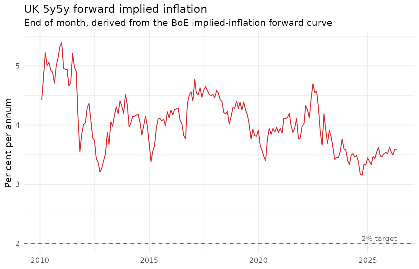
10-year UK nominal spot rate, 2000 to present

5y5y forward implied inflation

The 5y5y forward inflation rate (the average implied inflation rate over the second five-year horizon, five years from now) is a textbook medium-term inflation expectations measure. It comes straight off the implied-inflation forward curve.

inflation_fwd <- boe_curve_panel(
  curve     = "inflation",
  measure   = "forward",
  frequency = "monthly",
  from      = "2010-01-01",
  maturities = c(5, 10)
)
#> ℹ Downloading inflation monthly yield-curve archive from Bank of England
#> ✔ Downloading inflation monthly yield-curve archive from Bank of England [205ms]
#> 

inflation_fwd$five_y_five_y <- (inflation_fwd$m10 * 10 -
                                inflation_fwd$m5  *  5) / 5
head(inflation_fwd[, c("date", "m5", "m10", "five_y_five_y")])
#> # BoE: 6 obs
#>         date       m5      m10 five_y_five_y
#> 1 2010-01-31 3.299640 3.863640      4.427640
#> 2 2010-02-28 3.401710 4.095848      4.789986
#> 3 2010-03-31 3.415668 4.318069      5.220470
#> 4 2010-04-30 3.458722 4.233360      5.007998
#> 5 2010-05-31 2.957608 4.008686      5.059764
#> 6 2010-06-30 2.779321 3.854157      4.928993

if (requireNamespace("ggplot2", quietly = TRUE)) {
  ggplot2::ggplot(inflation_fwd, ggplot2::aes(date, five_y_five_y)) +
    ggplot2::geom_line(colour = "#d62728") +
    ggplot2::geom_hline(yintercept = 2.0, linetype = "dashed",
                        colour = "grey40") +
    ggplot2::annotate("text", x = max(inflation_fwd$date),
                      y = 2.0, label = "2% target", hjust = 1, vjust = -0.5,
                      colour = "grey40", size = 3) +
    ggplot2::labs(
      title    = "UK 5y5y forward implied inflation",
      subtitle = "End of month, derived from the BoE implied-inflation forward curve",
      x = NULL, y = "Per cent per annum"
    ) +
    ggplot2::theme_minimal()
}

UK 5y5y forward implied inflation, 2010 to present

OIS curve evolution across the rate cycle

The OIS curve gives a market-implied path for Bank Rate. Comparing OIS spot pillars at MPC decision dates shows how expectations shifted through the 2022 to 2024 hiking cycle.

ois <- boe_curve_panel(
  curve     = "ois",
  measure   = "spot",
  frequency = "monthly",
  from      = "2020-01-01",
  maturities = c(0.5, 1, 2, 5)
)
#> ℹ Downloading ois monthly yield-curve archive from Bank of England
#> ✔ Downloading ois monthly yield-curve archive from Bank of England [212ms]
#> 

mpc <- boe_mpc_decisions(from = "2020-01-01")
#> ℹ Downloading from Bank of England
#> ✔ Downloading from Bank of England [441ms]
#> 
mpc <- data.frame(date = mpc$date, bank_rate = mpc$new_rate_pct)

merged <- merge(ois, mpc, by = "date", all.x = TRUE)
merged$bank_rate <- as.numeric(merged$bank_rate)

# carry the bank rate forward between MPC dates
for (i in seq_along(merged$bank_rate)) {
  if (i > 1 && is.na(merged$bank_rate[i])) {
    merged$bank_rate[i] <- merged$bank_rate[i - 1]
  }
}
tail(merged)
#>          date     m0.5       m1       m2       m5 bank_rate
#> 70 2025-11-28 3.670990 3.533751 3.468765 3.589609        NA
#> 71 2025-12-31 3.613941 3.485618 3.454123 3.621165        NA
#> 72 2026-01-30 3.603969 3.491676 3.492607 3.727255        NA
#> 73 2026-02-27 3.461611 3.348672 3.309542 3.485201        NA
#> 74 2026-03-31 3.950747 4.102948 4.162256 4.106304        NA
#> 75 2026-04-30 3.968888 4.190262 4.258125 4.245096        NA

if (requireNamespace("ggplot2", quietly = TRUE)) {
  long <- data.frame(
    date  = rep(merged$date, 5),
    pillar = rep(c("Bank Rate", "6m OIS", "1y OIS", "2y OIS", "5y OIS"),
                 each = nrow(merged)),
    rate  = c(merged$bank_rate, merged$m0.5, merged$m1, merged$m2, merged$m5)
  )
  long$pillar <- factor(long$pillar,
                        levels = c("Bank Rate", "6m OIS", "1y OIS",
                                   "2y OIS", "5y OIS"))

  ggplot2::ggplot(long, ggplot2::aes(date, rate, colour = pillar)) +
    ggplot2::geom_line() +
    ggplot2::labs(
      title    = "UK OIS spot pillars and Bank Rate, 2020 to present",
      subtitle = "Tightening cycle visible across all pillars",
      x = NULL, y = "Per cent", colour = NULL
    ) +
    ggplot2::theme_minimal() +
    ggplot2::theme(legend.position = "bottom")
}
#> Warning: Removed 75 rows containing missing values or values outside the scale range
#> (`geom_line()`).

UK OIS spot pillars and Bank Rate, 2020 to present

When to reach for the archive

Question	Argument set
Today’s curve	none (default)
Last few years, daily	`from = "2020-01-01"`
Multi-decade panel for econometrics	`frequency = "monthly", from = "1990-01-01"`
Commercial bank liability curve	`curve = "blc"` (always uses archive)

Archive zips cache for 30 days by default; the latest-month zip caches for 24 hours. Override with cache_ttl_h if you need to force a fresh pull.

References

Anderson, N. and Sleath, J. (2001). New estimates of the UK real and nominal yield curves. Bank of England Working Paper No. 126. https://www.bankofengland.co.uk/working-paper/2001/new-estimates-of-the-uk-real-and-nominal-yield-curves