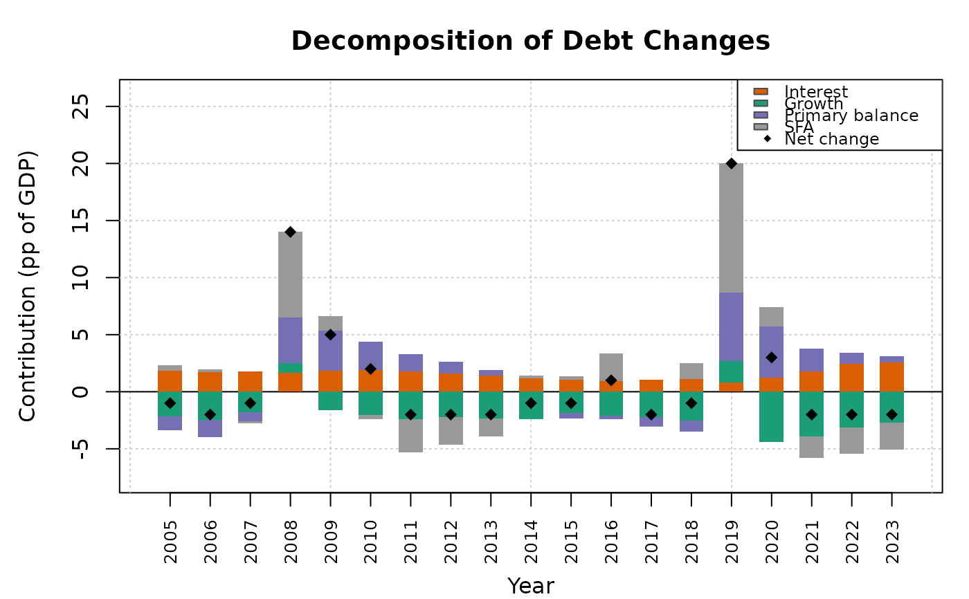
Decompose Historical Debt Changes — dk

Breaks down observed year-on-year changes in the debt-to-GDP ratio into four components:

Usage

dk_decompose(debt, interest_rate, gdp_growth, primary_balance, years = NULL)

Arguments

debt: Numeric vector of historical debt-to-GDP ratios.
interest_rate: Numeric vector of effective interest rates on government debt. Must be the same length as debt.
gdp_growth: Numeric vector of nominal GDP growth rates. Must be the same length as debt.
primary_balance: Numeric vector of primary balance-to-GDP ratios (positive = surplus). Must be the same length as debt.
years: Optional integer vector of year labels. Must be the same length as debt. If NULL (default), years are numbered sequentially.

Value

An S3 object of class dk_decomposition containing:

data: A data.frame with columns year, debt, change, interest_effect, growth_effect, snowball_effect, primary_balance_effect, and sfa.
years: The year labels used.

Details

Interest effect: \(r_t / (1 + g_t) \cdot d_{t-1}\)
Growth effect: \(-g_t / (1 + g_t) \cdot d_{t-1}\)
Primary balance effect: \(-pb_t\)
Stock-flow adjustment (residual): actual change minus the sum of the three identified components.

This is the standard decomposition used by the IMF (2013) and European Commission. The SFA residual captures privatisation receipts, exchange-rate valuation changes, below-the-line operations, and any measurement error.

References

Blanchard, O.J. (1990). Suggestions for a New Set of Fiscal Indicators. OECD Economics Department Working Papers, No. 79. doi:10.1787/budget-v2-art12-en

International Monetary Fund (2013). Staff Guidance Note for Public Debt Sustainability Analysis in Market-Access Countries. IMF Policy Paper.

Examples

d <- dk_sample_data()
dec <- dk_decompose(
  debt = d$debt,
  interest_rate = d$interest_rate,
  gdp_growth = d$gdp_growth,
  primary_balance = d$primary_balance,
  years = d$years
)
dec
#> 
#> ── Debt Decomposition ──────────────────────────────────────────────────────────
#> • Periods: 19 (2005–2023)
#> • Cumulative change: 24 pp
#> •  Interest effect: 29.8 pp
#> •  Growth effect: -39.5 pp
#> •  Primary balance: 20.9 pp
#> •  Stock-flow adj.: 12.8 pp
plot(dec)