Estimate trend inflation

Extracts the trend component from an inflation series using one of four methods: Hodrick-Prescott filter, Beveridge-Nelson decomposition, exponential smoothing, or centred moving average.

Usage

ik_trend(
  x,
  method = c("hp", "beveridge_nelson", "exponential_smooth", "moving_average"),
  frequency = c("quarterly", "monthly", "annual"),
  lambda = NULL,
  window = NULL
)

Arguments

x

Numeric vector. An inflation time series.

method

Character. One of "hp", "beveridge_nelson", "exponential_smooth", or "moving_average".

frequency

Character. Data frequency: "quarterly" (default), "monthly", or "annual". Used to set the HP filter lambda (when lambda = NULL) and moving average window (when window = NULL).

lambda

Numeric or NULL. Smoothing parameter for the HP filter. If NULL, defaults based on frequency: 6.25 for annual, 1600 for quarterly (Hodrick and Prescott, 1997), or 14400 for monthly (Backus and Kehoe, 1992).

window

Integer or NULL. Window size for the moving average method. Defaults to 4 for quarterly, 12 for monthly, or 3 for annual.

Value

An S3 object of class "ik_trend" with elements:

trend

Numeric vector. The estimated trend component.

cycle

Numeric vector. The cyclical component (original minus trend).

method

Character. The method used.

lambda

Numeric. HP filter lambda (if applicable).

window

Integer. Moving average window (if applicable).

alpha

Numeric. Exponential smoothing parameter (if applicable).

original

Numeric vector. The original series.

References

Hodrick, R. J. and Prescott, E. C. (1997). "Postwar U.S. Business Cycles: An Empirical Investigation." Journal of Money, Credit and Banking, 29(1), 1-16.

Ravn, M. O. and Uhlig, H. (2002). "On Adjusting the Hodrick-Prescott Filter for the Frequency of Observations." Review of Economics and Statistics, 84(2), 371-376.

Examples

data <- ik_sample_data("headline")
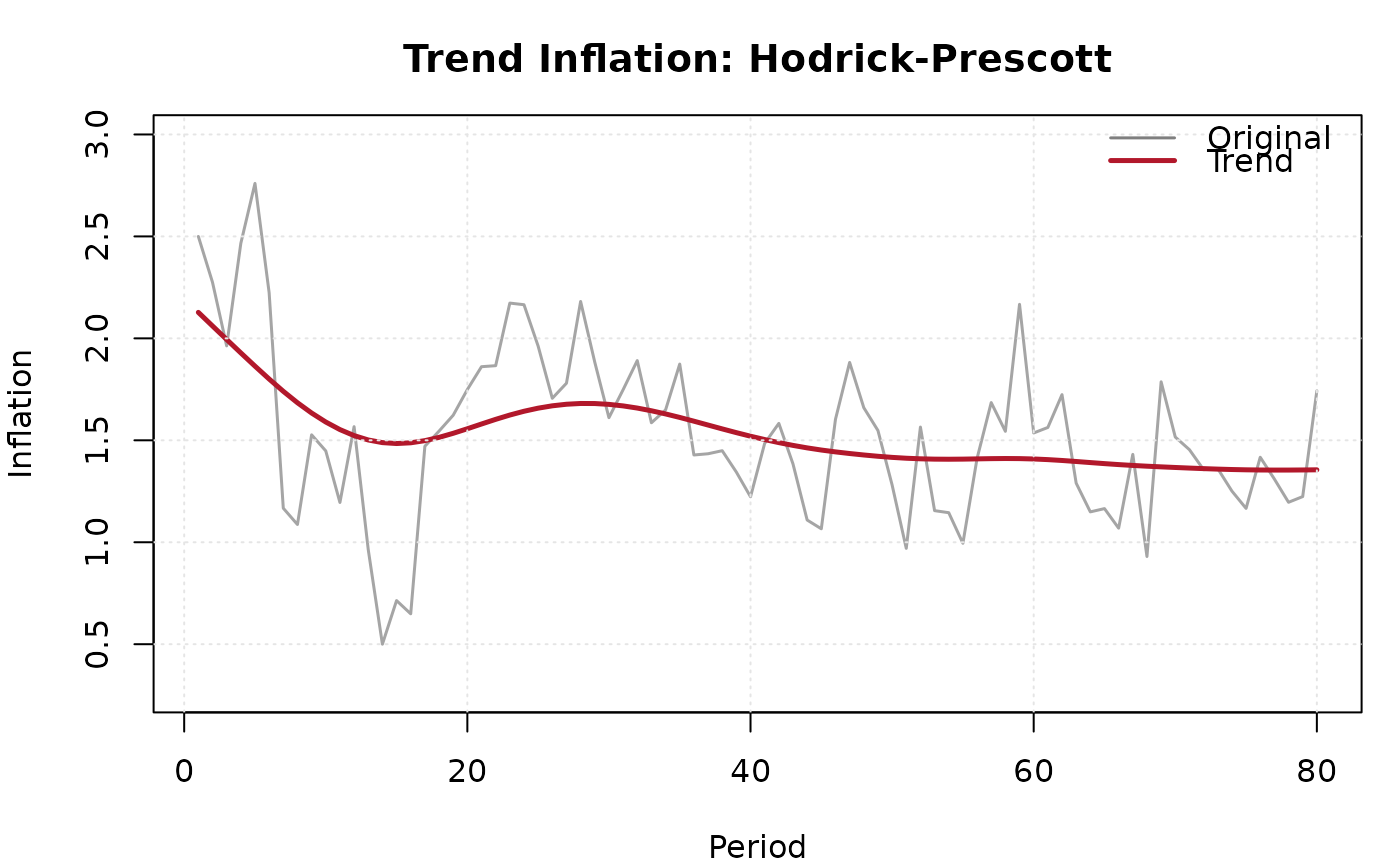
tr <- ik_trend(data$inflation, method = "hp")
print(tr)
#> 
#> ── Trend Inflation ─────────────────────────────────────────────────────────────
#> • Method: Hodrick-Prescott (lambda = 1600)
#> • Mean trend: 1.5261
#> • Cycle volatility (SD): 0.3405
#> • Observations: 80
plot(tr)


tr_ma <- ik_trend(data$inflation, method = "moving_average", window = 4)
print(tr_ma)
#> 
#> ── Trend Inflation ─────────────────────────────────────────────────────────────
#> • Method: Moving Average (window = 4)
#> • Mean trend: 1.5298
#> • Cycle volatility (SD): 0.2118
#> • Observations: 80