Chapter 3 Making maps with python

Maps are a great way to communicate data. They’re easily understandable, flexible, and more intuitive than a chart. There’s been numerous studies showing that the average professional often struggles to interpret the units on a y-axis, let alone understand trends in scatter or line graphs.

Making maps in R takes some initial investment (note: they can be fiddly). However once you have some code you know and understand, spinning up new pieces of analysis can happen in minutes, rather than hours or days.

The aim of this quick-reference guide is to get you from ‘I can produce a map in R’ to something more like ‘I can conduct spatial analysis and produce a visual which is ready to send without any further work.’

knitr::opts_chunk$set(echo = TRUE)

library(reticulate)

# py_install is a special wrapper from the reticulate package that does "conda install" automatically

use_condaenv("tf")

reticulate::py_install("geopy")

reticulate::py_install("geocoder")

3.1 Importing python packages

Let’s load in some libraries that we will use again and again when making charts.

import matplotlib.pyplot as plt
import matplotlib.dates as mdates
import pandas as pd
import geopandas as gpd
import numpy as np
import statistics

from scipy.stats import norm
from matplotlib.ticker import EngFormatter, StrMethodFormatter

3.2 Making simple maps with geopandas

Just like a pandas dataframe, the geopandas package allows us to us shapefiles.

We’ll go ahead and download some shapefiles from the ABS.

# Read the SHP file
SA4_shp = gpd.read_file('ASGS/SA4_2021_AUST_SHP_GDA2020/SA4_2021_AUST_GDA2020.shp')    

# Load the data using Geopandas
SA4_shp.head()

# Check the coordinate reference system attached to the shapefile

SA4_shp.crs

# Filter the data for only Greater Melbourne

SA4_shp_MEL = SA4_shp[SA4_shp['GCC_NAME21']=='Greater Melbourne'] 
SA4_shp_MEL.head()

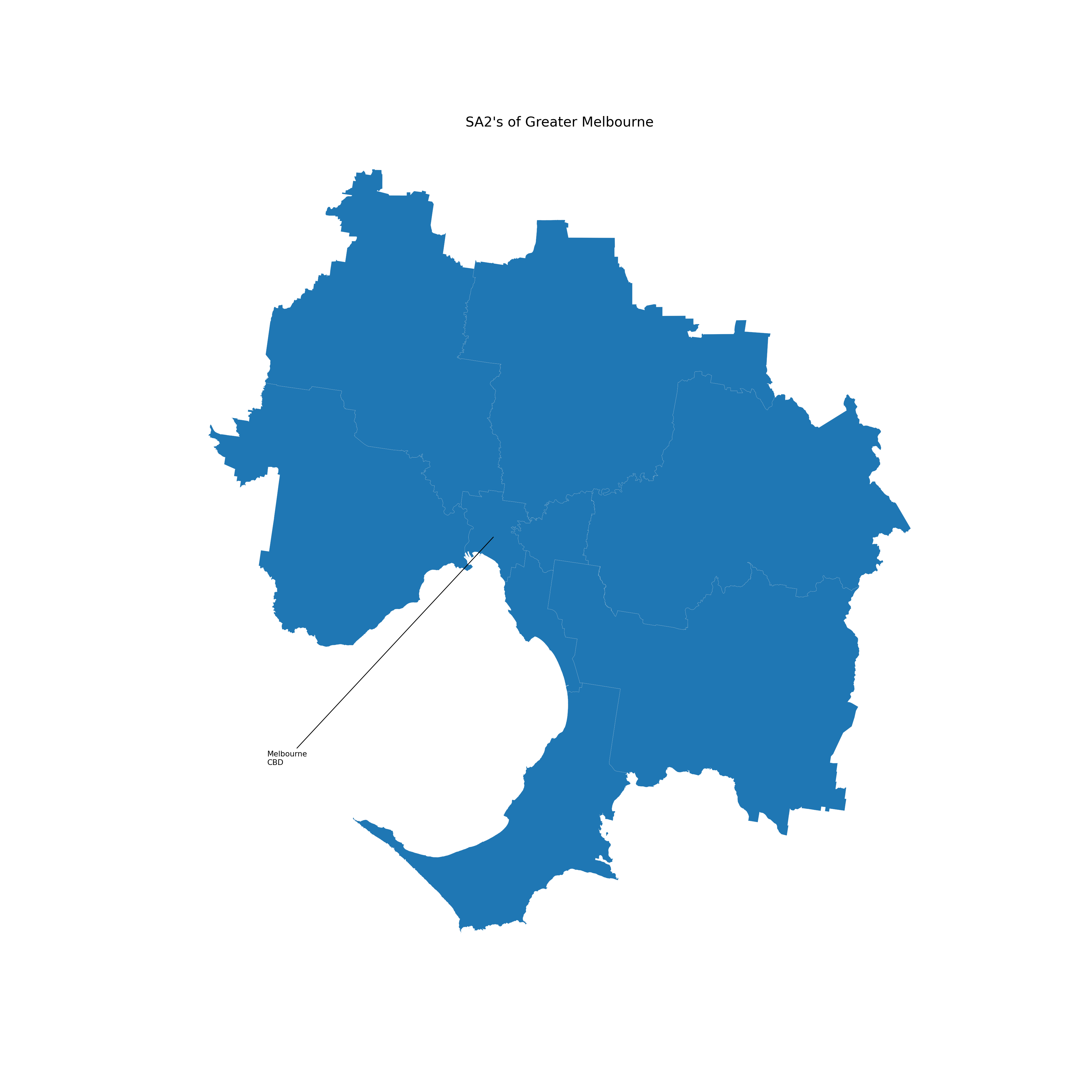
# Quick plot of the shapefile

SA4_shp_MEL.plot(figsize=(20, 20), linewidth=0.1, edgecolor='0.9', legend = True)

plt.annotate('Melbourne\nCBD',
            xy=(144.96246,-37.81214),
            xytext=(144.46246,-38.21),
            arrowprops = dict(arrowstyle='-'))

plt.title("SA2's of Greater Melbourne", fontsize=18)

plt.gca().axis('off')

plt.show()

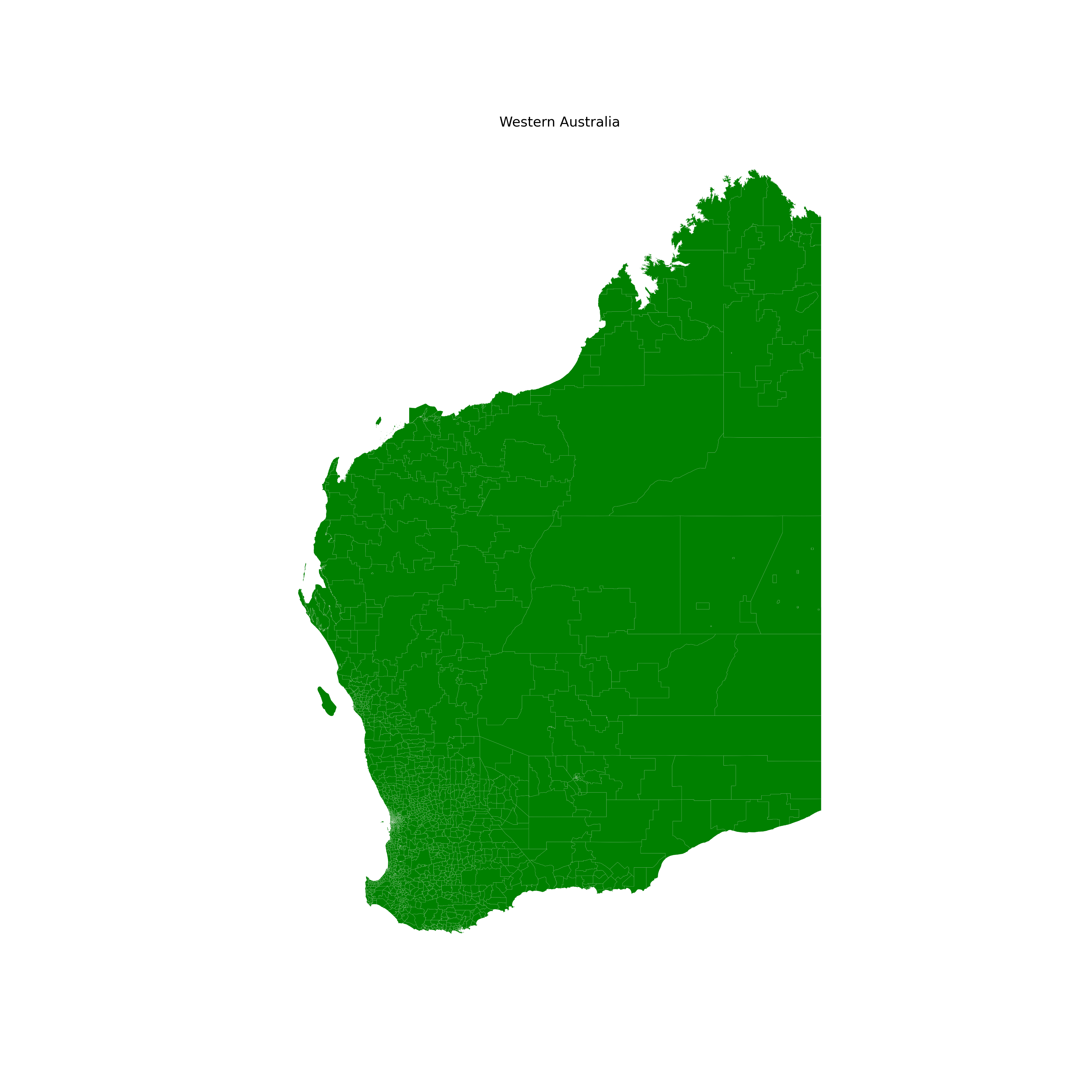
Here’s another example using a shapefile for WA

# Load Geometry File
WA_shp = gpd.read_file('data/NOV21_WA_LOC_POLYGON_shp_GDA2020/wa_localities.shp')    

WA_shp.plot(figsize=(20, 20), linewidth=0.1, color='green', edgecolor='0.9', legend = True)

plt.title("Western Australia", fontsize=18)

plt.gca().axis('off')

plt.show()

3.3 Geocoding address data

Using Nominatim to find the coordinates of a street address

from geopy.geocoders import Nominatim

geolocator = Nominatim(user_agent="coverdale")
test_location = geolocator.geocode("150 Collins Street, Melbourne Australia")

print(test_location.address)

print(test_location.latitude, test_location.longitude)

print(test_location.raw)

Using Nominatim to find the street address from a set of coordinates

from geopy.geocoders import Nominatim
geolocator = Nominatim(user_agent="coverdale")

test_location = geolocator.reverse("-37.81214, 144.96246")

print(test_location.address)

print(test_location.latitude, test_location.longitude)

print(test_location.raw)

We can also use geopy to find the distance between two points

Geopy can calculate geodesic distance between two points using the geodesic distance or the great-circle distance, with a default of the geodesic distance available as the function geopy.distance.distance.

#Here's an example usage of the geodesic distance:
from geopy.distance import geodesic
sydney = (-37.81214, 144.96246)
melbourne = (-33.8688, 151.2093)
print(geodesic(sydney, melbourne).kilometers)

# Using great-circle distance:

from geopy.distance import great_circle
sydney = (-37.81214, 144.96246)
melbourne = (-33.8688, 151.2093)
print(great_circle(sydney, melbourne).kilometers)

Note we see a slight difference in the km measurement (around 500m) - this is due to the earth not being exactly spherical.

Geocoding a list of addresses

hospital_data_clean = hospital_data.dropna()

# Split out the points into latitude and longitude

hospital_data_clean[[‘lat,’ ‘lon,’ ‘altitude’]] = pd.DataFrame(hospital_data[‘point’].to_list(), index=hospital_data.index)

# View dataframe

hospital_data_clean.head(5)

# Import necessary modules
import geopy
import geocoder
import geopandas as gpd
from shapely.geometry import Point
from geopandas.tools import geocode
from geopy.geocoders import Nominatim

geolocator = Nominatim(user_agent="coverdale")

from geopy.extra.rate_limiter import RateLimiter
geocode = RateLimiter(geolocator.geocode, min_delay_seconds=1)

# Read the data
hospital_data = pd.read_csv("data/QLD_public_hospitals.csv",
                on_bad_lines='skip',
                encoding='unicode_escape')
                
hospital_data.head(5)

# Add the state and country to the data

hospital_data['Address'] = hospital_data['Address'].astype(str) + ", Queensland, Australia"

# Find the location
hospital_data['location'] = hospital_data['Address'].apply(geocode)

# Turn the location into a point

hospital_data['point'] = hospital_data['location'].apply(lambda loc: tuple(loc.point) if loc else None)

hospital_data_clean = hospital_data.dropna()

# Split out the points into latitude and longitude
hospital_data_clean[['lat', 'lon', 'altitude']] = pd.DataFrame(hospital_data_clean['point'].to_list(), index=hospital_data_clean.index)

geometry = [Point(xy) for xy in zip (hospital_data_clean['lon'], hospital_data_clean['lat'])]

hospital_geodataframe = gpd.GeoDataFrame(hospital_data_clean,
                                        crs="EPSG:4326", 
                                        geometry=geometry)

#hospital_geodataframe.set_crs(epsg=4326, inplace=True)

# View dataframe
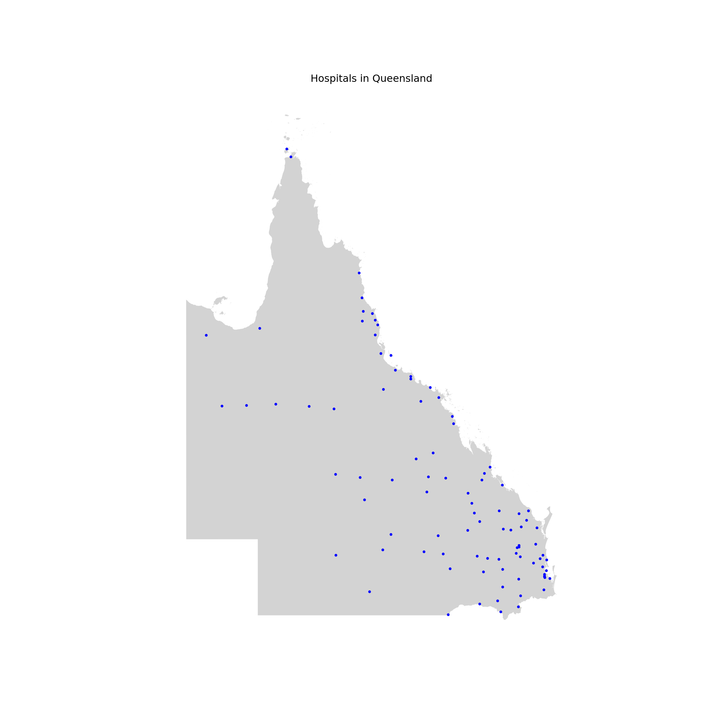
hospital_geodataframe.head(5)

Let’s now plot these points on a map of Queensland. We’ll also need to load in the shape of Queensland as the ‘base map.’

# Read the SHP file
STE_shp = gpd.read_file('ASGS/STE_2021_AUST_SHP_GDA2020/STE_2021_AUST_GDA2020.shp')    

# Load the data using Geopandas
STE_shp.head()

# Check the coordinate reference system attached to the shapefile

STE_shp.crs

# Filter the data for only Greater Melbourne

STE_shp_QLD = STE_shp[STE_shp['STE_NAME21']=='Queensland'] 
STE_shp_QLD.head()

Now we plot the two layers together

fig, ax = plt.subplots(1, 1, figsize=(12, 12))

# Base layer with all the areas for the background
STE_shp_QLD.plot(ax=ax, linewidth=0.1, color='lightgrey', edgecolor='0.9')

# Hospital points
hospital_geodataframe.plot(ax=ax, alpha=1, facecolor='blue', markersize=5)

plt.title("Hospitals in Queensland", fontsize=12)

ax.set_axis_off()
plt.show()