Chapter 9 Web-scraping
9.1 Introduction
Getting content off websites can be a nightmare. The worst case resort is manually typing data from a web-page into spreadsheets… but there are many steps we can do before resorting to that.
This chapter will outline the process for pulling data off the web, and particularly for understanding the exact web-page element we want to extract. The notes and code loosely follow the fabulous tutorial by Grant R. McDermott in his Data Science for Economistsseries.
First up, let’s load some packages.
# Load and install the packages
pacman::p_load(tidyverse, dplyr, rvest, lubridate, janitor, data.table, hrbrthemes)
9.2 Anatomy of a webpage
Let’s introduce some terminology: server side
This describes information being embeded directly in the webpage’s HTML. When dealing with server side webpages, finding the correct CSS (or Xpath) “selectors” becomes the hardest part of the task.
Iterating through dynamic webpages (e.g. “Next page” and “Show More” tabs) is also tricky - but we’ll get there.
Trawling through CSS code on a webpage is a bit of a nightmare - so we’ll use a chrome extension called SelectGadget to help.
The R package that’s going to do the heavy lifting is called rvest and is based on the python package called Beauty Soup.
9.3 Scraping a table
Let’s use this wikipedia page as a starting example. It contains various entries for the men’s 100m running record.
We can start by pulling all the data from the webpage.
m100 <- rvest:: read_html("https://en.wikipedia.org/wiki/Men%27s_100_metres_world_record_progression")
m100
## {html_document}
## <html class="client-nojs" lang="en" dir="ltr">
## [1] <head>\n<meta http-equiv="Content-Type" content="text/html; charset=UTF-8 ...
## [2] <body class="mediawiki ltr sitedir-ltr mw-hide-empty-elt ns-0 ns-subject ...…and we get a whole heap of mumbo jumbo.
To get the table of ‘Unofficial progression before the IAAF’ we’re going to have to be more specific.
Using the SelectGadget tool we can click around and identify that that specific table is named in the HTML code: .wikitable :nth-child(1)
Side note: The names of tables in HTML webpages changes all the time. Therefore this code is considered unstable in terms of setting and forgetting.
pre_iaaf <-
  m100 %>%
  #Select table
  rvest::html_element(".wikitable :nth-child(1)") %>%
  #Convert to data frame
  rvest::html_table()

pre_iaaf
## # A tibble: 21 x 5
## Time Athlete Nationality `Location of races` Date
## <dbl> <chr> <chr> <chr> <chr>
## 1 10.8 Luther Cary United States Paris, France July 4, 1~
## 2 10.8 Cecil Lee United Kingdom Brussels, Belgium September~
## 3 10.8 Étienne De Ré Belgium Brussels, Belgium August 4,~
## 4 10.8 L. Atcherley United Kingdom Frankfurt/Main, Germany April 13,~
## 5 10.8 Harry Beaton United Kingdom Rotterdam, Netherlands August 28~
## 6 10.8 Harald Anderson-Arbin Sweden Helsingborg, Sweden August 9,~
## 7 10.8 Isaac Westergren Sweden Gävle, Sweden September~
## 8 10.8 Isaac Westergren Sweden Gävle, Sweden September~
## 9 10.8 Frank Jarvis United States Paris, France July 14, ~
## 10 10.8 Walter Tewksbury United States Paris, France July 14, ~
## # ... with 11 more rowsNiiiiice - now that’s better. Let’s do some quick data cleaning.
pre_iaaf <- pre_iaaf %>%
            clean_names() %>%
            dplyr::mutate(date = mdy(date))

pre_iaaf
## # A tibble: 21 x 5
## time athlete nationality location_of_races date
## <dbl> <chr> <chr> <chr> <date>
## 1 10.8 Luther Cary United States Paris, France 1891-07-04
## 2 10.8 Cecil Lee United Kingdom Brussels, Belgium 1892-09-25
## 3 10.8 Étienne De Ré Belgium Brussels, Belgium 1893-08-04
## 4 10.8 L. Atcherley United Kingdom Frankfurt/Main, Germany 1895-04-13
## 5 10.8 Harry Beaton United Kingdom Rotterdam, Netherlands 1895-08-28
## 6 10.8 Harald Anderson-Arbin Sweden Helsingborg, Sweden 1896-08-09
## 7 10.8 Isaac Westergren Sweden Gävle, Sweden 1898-09-11
## 8 10.8 Isaac Westergren Sweden Gävle, Sweden 1899-09-10
## 9 10.8 Frank Jarvis United States Paris, France 1900-07-14
## 10 10.8 Walter Tewksbury United States Paris, France 1900-07-14
## # ... with 11 more rowsLet’s also scrape the data for the more recent running records. That’s the tables called ‘Pre-automatic timing (1912–1976),’ and ‘Modern Era (1977 onwards).’
For the second table:
iaaf_76 <- m100 %>%
           html_element("h3+ .wikitable") %>%
           rvest::html_table()

iaaf_76 <- iaaf_76 %>%
           clean_names() %>%
           mutate(date = mdy(date))

iaaf_76
## # A tibble: 54 x 8
## time wind auto athlete nationality location_of_race date ref
## <dbl> <chr> <dbl> <chr> <chr> <chr> <date> <chr>
## 1 10.6 "" NA Donald Lippi~ United Sta~ Stockholm, Swed~ 1912-07-06 [2]
## 2 10.6 "" NA Jackson Scho~ United Sta~ Stockholm, Swed~ 1920-09-16 [2]
## 3 10.4 "" NA Charley Padd~ United Sta~ Redlands, USA 1921-04-23 [2]
## 4 10.4 "0.0" NA Eddie Tolan United Sta~ Stockholm, Swed~ 1929-08-08 [2]
## 5 10.4 "" NA Eddie Tolan United Sta~ Copenhagen, Den~ 1929-08-25 [2]
## 6 10.3 "" NA Percy Willia~ Canada Toronto, Canada 1930-08-09 [2]
## 7 10.3 "0.4" 10.4 Eddie Tolan United Sta~ Los Angeles, USA 1932-08-01 [2]
## 8 10.3 "" NA Ralph Metcal~ United Sta~ Budapest, Hunga~ 1933-08-12 [2]
## 9 10.3 "" NA Eulace Peaco~ United Sta~ Oslo, Norway 1934-08-06 [2]
## 10 10.3 "" NA Chris Berger Netherlands Amsterdam, Neth~ 1934-08-26 [2]
## # ... with 44 more rowsAnd now for the third table:
iaaf <- m100 %>%
        html_element("p+ .wikitable") %>%
        html_table() %>%
        clean_names() %>%
        mutate(date = mdy(date))
iaaf
## # A tibble: 24 x 9
## time wind auto athlete nationality location_of_race date
## <dbl> <chr> <dbl> <chr> <chr> <chr> <date>
## 1 10.1 1.3 NA Bob Hayes United States Tokyo, Japan 1964-10-15
## 2 10.0 0.8 NA Jim Hines United States Sacramento, USA 1968-06-20
## 3 10.0 2.0 NA Charles Greene United States Mexico City, Mexico 1968-10-13
## 4 9.95 0.3 NA Jim Hines United States Mexico City, Mexico 1968-10-14
## 5 9.93 1.4 NA Calvin Smith United States Colorado Springs, ~ 1983-07-03
## 6 9.83 1.0 NA Ben Johnson Canada Rome, Italy 1987-08-30
## 7 9.93 1.0 NA Carl Lewis United States Rome, Italy 1987-08-30
## 8 9.93 1.1 NA Carl Lewis United States Zürich, Switzerland 1988-08-17
## 9 9.79 1.1 NA Ben Johnson Canada Seoul, South Korea 1988-09-24
## 10 9.92 1.1 NA Carl Lewis United States Seoul, South Korea 1988-09-24
## # ... with 14 more rows, and 2 more variables: notes_note_2 <chr>,
## # duration_of_record <chr>How good. Now let’s bind the rows together to make a master data set.
wr100 <- rbind(
    pre_iaaf %>% dplyr::select(time, athlete, nationality, date) %>%
    mutate(era = "Pre-IAAF"),
    iaaf_76 %>% dplyr::select(time, athlete, nationality, date) %>%
    mutate(era = "Pre-automatic"),
    iaaf %>% dplyr::select(time, athlete, nationality, date) %>%
    mutate(era = "Modern")
    )

wr100
## # A tibble: 99 x 5
## time athlete nationality date era
## <dbl> <chr> <chr> <date> <chr>
## 1 10.8 Luther Cary United States 1891-07-04 Pre-IAAF
## 2 10.8 Cecil Lee United Kingdom 1892-09-25 Pre-IAAF
## 3 10.8 Étienne De Ré Belgium 1893-08-04 Pre-IAAF
## 4 10.8 L. Atcherley United Kingdom 1895-04-13 Pre-IAAF
## 5 10.8 Harry Beaton United Kingdom 1895-08-28 Pre-IAAF
## 6 10.8 Harald Anderson-Arbin Sweden 1896-08-09 Pre-IAAF
## 7 10.8 Isaac Westergren Sweden 1898-09-11 Pre-IAAF
## 8 10.8 Isaac Westergren Sweden 1899-09-10 Pre-IAAF
## 9 10.8 Frank Jarvis United States 1900-07-14 Pre-IAAF
## 10 10.8 Walter Tewksbury United States 1900-07-14 Pre-IAAF
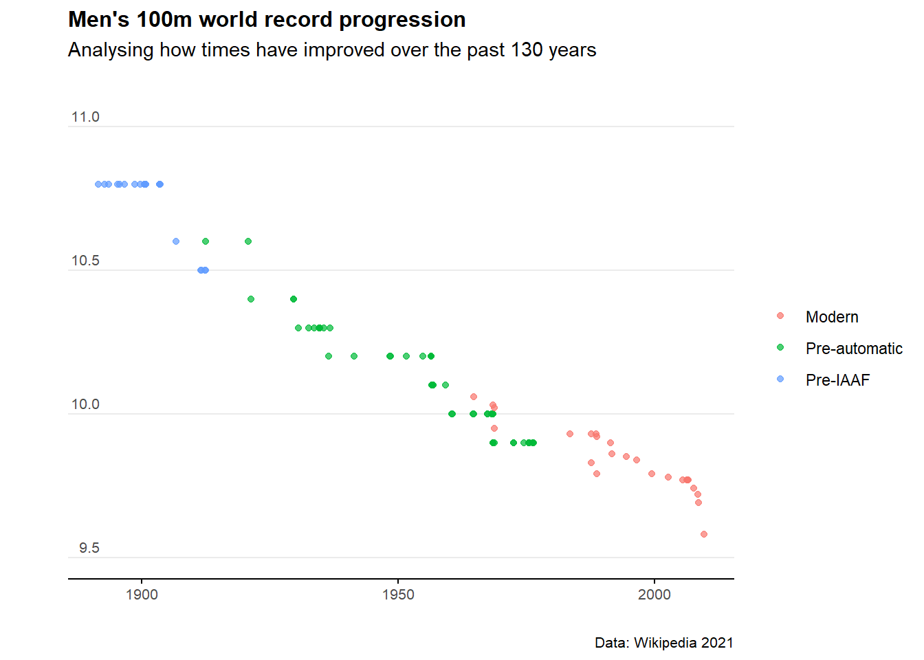
## # ... with 89 more rowsExcellent. Let’s plot the results.
ggplot(wr100)+
  geom_point(aes(x = date, y = time, col = era),alpha=0.7)+

  labs(title="Men's 100m world record progression",
  subtitle = "Analysing how times have improved over the past 130 years",
  caption = "Data: Wikipedia 2021",
  x="",
  y="") +

  theme_minimal()+

  scale_y_continuous(limits=c(9.5,11), breaks=c(9.5,10,10.5,11))+

  theme(axis.text.y = element_text(vjust = -0.5, margin = ggplot2::margin(l = 20, r = -20)))+

  theme(plot.subtitle = element_text(margin=ggplot2::margin(0,0,25,0))) +

  theme(legend.title = element_blank())+

  theme(plot.title=element_text(face="bold",size=12))+
  theme(plot.subtitle=element_text(size=11))+
  theme(plot.caption=element_text(size=8))+

  theme(axis.text=element_text(size=8))+
  theme(panel.grid.minor = element_blank())+
  theme(panel.grid.major.x = element_blank()) +

  theme(axis.line.x = element_line(colour ="black",size=0.4))+
  theme(axis.ticks.x = element_line(colour ="black",size=0.4))